Testing a non-linearity correction using the ratio method

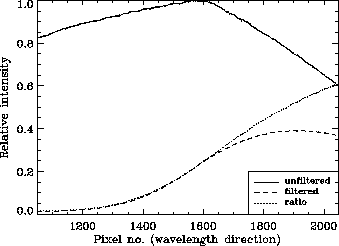
Ratio measurements from spectra were made in 1997, using a colour filter to cover half of the length of the slit. The aim was to check the validity of the non-linearity curve of CCD10 derived using the BRE method (Section 2.1). Figure 2 shows two cross-sections of a flat-field image from a filtered and an un-filtered part and the ratio between the two parts.

Figure 2: Cross-sections of flat-field image used for the ratio method. The solid line represents the direct spectrum of the lamp with vignetting above pixel 1600. The dashed line represents a parallel cross-section where the light has passed through a colour filter. The dotted line represents the transmission profile of the filter. The wavelength range is around 6600-7000Å but this is not important as far as non-linearity measurements are concerned.

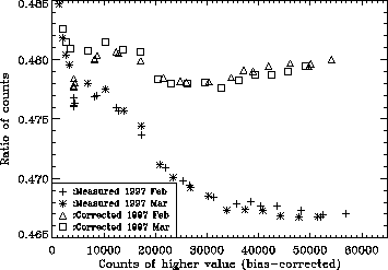
In Figure 3, the ratios between filtered and un-filtered parts of the flat-field versus counts of the un-filtered part are plotted, using two sets of exposures. In Figure 4, the ratios are plotted for a different wavelength using the same exposures. There is clearly a decrease in the measured ratio at higher light levels due to the non-linearity of the CCD. This is consistent with an increase in the relative gain of the CCD at higher light levels, as seen using the BRE method.

Figure 3: Testing of non-linearity curve of CCD10 using ratio method. The measurements (crosses and asterisks) represent intensity ratios between a filtered and unfiltered part of a flat-field image (see Fig. 2; with measurements around pixel no. 1450 for this figure, and 1850 for Fig. 4). Each measurement is taken from a different exposure. The corrected ratios (triangles and squares) are recalculated after applying the non-linearity correction given in Eqn. 1.

Figure 4: Testing of non-linearity curve of CCD10. See Fig. 3 for details.

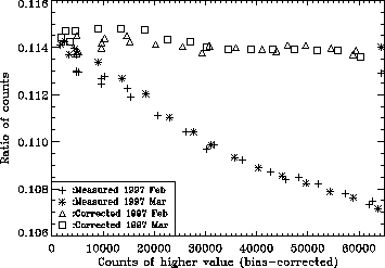Additionally, the data were corrected for non-linearities using the quadratic fit given in Equation 1 and the ratios were re-calculated. These corrected ratios are also shown in Figures 3-4. There is a definite improvement in the `ratio variation' by a factor of about 5 after the non-linearity correction has been made.

This ratio method has a very low scatter and seems to be detecting higher order non-linearities which were not evident using the BRE method. Note that at light levels below 10000 counts, the scatter is much higher, probably because of errors in bias subtraction. Structure in the non-linearity curve appears around 18000 and 31000 counts, as is most evident in Figure 4. It is likely that the BRE method has smoothed over these high-order changes because of the normalisation and the scatter in the plots. Despite these glitches, the 2nd order fit derived by the BRE method has improved the non-linearity significantly and, therefore, it was valuable to use this non-linearity correction on data obtained with this CCD.

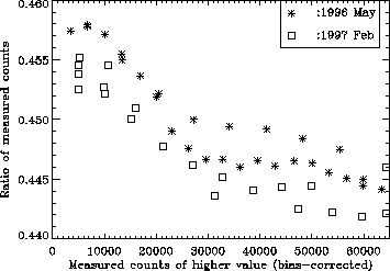
We have also tested the stability of the non-linearity correction over time by comparing flat fields taken in 1996 with some taken in 1997. Figure 5 shows this comparison using the ratio method. Notably, the shape of the ratio variation with count level is similar implying that the non-linearity had not changed significantly.

Figure 5: Comparison of non-linearity data of CCD10 using ratio method. This figure demonstrates that the non-linear properties of the CCD were similar in 1996 and 1997. Ignore the fact that the mean ratio is different between the two years, that is not due to non-linearity, and that the scatter is higher than in the previous figures, the ratio was measured between two different wavelengths of a flat field image because no colour filter was used in 1996. The significant fact is that the shape of the ratio variation is similar.