Measurement of non-linearity using the ratio method

The ratio method can be used to determine a non-linearity curve, for example, by solving an equation of the form

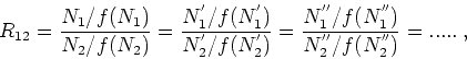$$R_{12} = \frac{ N_1 / f( N_1 ) }{ N_2 / f( N_2 ) } = \frac{... ...''} / f( N_1^{''} ) }{ N_2^{''} / f( N_2^{''} ) } = ..... \: ,$$ (2)

where $N_1$ and $N_2$ are the measured counts of the two regions, at different light levels $N$ $N^{'}$ $N^{''}$ etc., $f(N)$ is the non-linearity function equivalent to measured-counts / expected-counts and, $R_{12}$ is the ratio of the expected (or true) counts between the two regions (the corrected ratio). A fit can be made to the parameters chosen for the non-linearity function, by minimising the scatter in the corrected ratio between different light levels. Similar equations can be solved for different pairs of regions on the CCD. For low intensity non-linearity tests, it will be necessary to obtain a good over-scan region for accurate bias subtraction.

In 1998 December, we observed at Mt. Stromlo using CCD17 (2Kx4K SITe with a nominal gain of 2.5e$^-$/ADU and 1x2 binning). We measured the non-linearity of this CCD using the ratio method.

Barton (1986) described the AAO CCD non-linearities in terms of an $\alpha$ parameter (see also Gilliland et al. 1993, Leach et al. 1980 and Tinney 1996), similar to $\alpha$ in the equation:

$$\frac{N_m}{N_t} = 1 + \alpha N_m$$ (3)

where $N_m$ are the measured counts in ADU above the bias level and $N_t$ are the `true counts' (normalised so that $N_t = N_m$ for $N_m \rightarrow 0$). The non-linearity of CCD17 was assumed to be represented by this single parameter. For high sensitivity to this parameter when using the ratio method, $R_{12}$ should be in the range 0.15-0.45.

For each set of ratio measurements, $\alpha$ was varied until the best fit for the corrected ratios had a slope of zero. The fit was obtained using the ratios with counts of the higher-value between 0 and 40000. Lower weight was given to those with counts below 10000 because of increased noise. Figures 6-8 show the value of $\alpha$ and the corrected ratios, for three sets of measurements. For CCD17, $\alpha$ is about $-3.5 \times 10^{-7}$.

Figure 6: Non-linearity measurement of CCD17 using ratio method. The squares represent the measured ratios, while the asterisks represent the ratios after correcting the intensities using the alpha parameter [ $N_t = N_m / (1 + \alpha N_m)$]. The lines are best fits to each set of ratios, between 0 and 40000 counts, with lower weight given to measurements below 10000. The alpha value has been chosen so that the slope of the best fit to the corrected ratios is zero.

Figure 7: Non-linearity measurement of CCD17. See Fig. 6 for details.

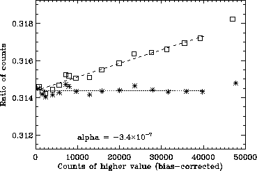Figure 8: Non-linearity measurement of CCD17. See Fig. 6 for details.

The ratio method removes the problems of requiring accurate exposure times and lamp-temperature stability to make accurate non-linearity measurements. Improvement of the accuracy of the method described in this section could be made by (i) taking more exposures, (ii) increasing and decreasing the exposure time several times, and (iii) interspersing the exposures with bias frames. In the second case, this will reduce problems which might arise from a systematic change in the measurements with time. In the third case, monitoring any changes in bias frames will improve the accuracy of bias subtraction which is critical for measurements with low counts.