Logarithmic shift zeta

Determining redshifts by cross correlation makes it evident that a `redshift' or velocity measurement is actually a shift on a logarithmic wavelength scale (Tonry & Davis, 1979). So arguably it is more natural to define a quantity (here called zeta) that is a logarithmic shift as

$$\zeta \: = \: \ln \lambda_{\rm obs} - \ln \lambda_{\rm em} \: = \: \ln (1+z)$$ (7)

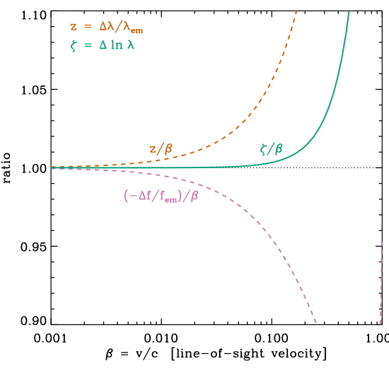
First we check its approximation for velocity, using Taylor series,

$$\begin{split} \zeta_{\rm pec} & = \: -\frac{1}{2} \ln({1-\bet... ... \beta_{\rm los}^2) + \frac{1}{3} \beta_{\rm los}^3 \end{split}$$ (8)

from the natural logarithm of Eq. 5. Such that $\zeta_{\rm pec}$ is always a more accurate approximation for $\beta_{\rm los}$ than $z_{\rm pec}$, with the quadratic term vanishing for pure line-of-sight motion. Figure 1 shows a comparison between the redshift, zeta and `radio definition' approximations for recession velocity.

Figure 1: Comparison between approximations for recession velocity, i.e., assuming pure line-of-sight motion ( $\beta _{\rm los} = \beta$). The Doppler formula is used to compute the redshift (Eq. 5), zeta (Eq. 7) and the radio definition of velocity as a function of $\beta$. Notably zeta remains an accurate approximation of recession velocity, within a percent, up to $0.1\,c$.

Given the improved accuracy, it is reasonable to use

$$\zeta_{\rm pec} \: \simeq \: \frac{v}{c}$$ (9)

for peculiar velocities. This is used implicitly when velocity dispersions of galaxies are determined from a logarithmically binned wavelength scale (Simkin, 1974).

More importantly, the use of zeta means that, the equivalent of Eq. 3 for relating redshift terms becomes

$$\zeta_{\rm cmb} \: = \: \zeta_{\rm helio} + \zeta_{\rm pec,\odot} \: = \: \zeta_{\rm cos} + \zeta_{\rm pec}$$ (10)

It is immediately evident that the separation in zeta between two galaxies at the same distance is related to velocity directly by

$$\Delta \zeta \: \simeq \: \frac{\Delta v}{c}$$ (11)

with no dependence on the choice of frame or cosmological redshift. In addition to being more accurate than Eq. 4, it is precisely symmetric when determining the separations in velocity between two or more galaxies, i.e., there is no need to pick a fiducial redshift. A velocity dispersion is given by $\sigma(\zeta)$ regardless of the frame.

Redshift measurement errors can also be addressed as follows. Spectroscopic or photometric redshifts are generally estimated by matching a template to a set of observed fluxes at different wavelengths. In order to determine the redshift, the template must be shifted in $\ln \lambda$, thus we can immediately see that:

$$\sigma(\zeta) \: = \: \sigma[\Delta \ln(\lambda)]$$ (12)

which is the uncertainty in the logarithmic shift between the observed and emitted wavelengths. Alternatively the redshift uncertainties are often quoted in fractional form:

$$\sigma(\zeta) \: \simeq \: \frac{\sigma(z)}{1+z}$$ (13)

Either can be related to a velocity uncertainty (Eq. 11), and it is thus reasonable to quote spectroscopic measurements using velocity uncertainties (Baldry et al., 2014). The concern is that some papers quote redshift errors in km/s using $\sigma(z)\,c$ (e.g. Colless et al. 2001), which does not represent a physical velocity uncertainty even though it has the same units.

It is appropriate to treat the evaluation of photometric redshift errors in the same way and determine the uncertainties in $\zeta$. The typical use of quoting ${\sigma(z)}/(1+z_{\rm spec})$, where $z_{\rm spec}$ is a spectroscopic redshift, for the performance of photometric redshift estimates, approximates this (e.g. Brinchmann et al. 2017). This is somewhat inelegant because the uncertainties on photometric redshifts are obtained using spectroscopic redshifts in the denominator. This is no such problem using $\sigma(\zeta)$ and it is more natural since a measurement corresponds to a shift in $\ln \lambda$. This is just a recognition that fractional differences between two quantities ($1 + z$ in this case) depend on a fiducial value whereas logarithmic differences are symmetric. More importantly, this strongly suggests that probability distribution functions, for example, should be assessed as a function of zeta (binning, outliers, biases, second peak offsets) rather than $z$. Rowan-Robinson (2003) used $\log_{10}(1+z)$, which equals $\zeta / \ln(10)$, in his analysis including plots but this is far from standard in the literature.